REPEATER SYSTEMS : Cavity resonators and duplexers

Cavity Resonators

Receiver desensing can be reduced by separating the transmitter and receiver antennas. But the amount of transmitted energy that reaches the receiver input must often be decreased even farther. Other nearby transmitters can cause desensing as well. A cavity resonator (cavity filter) can be helpful in solving these problems.

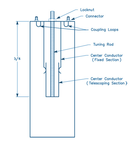
When properly designed and constructed, this type of resonator has very high Q. A cavity resonator placed in series with a transmission line acts as a band-pass filter. For a resonator to operate in series, it must have input and output coupling loops (or probes). A cavity resonator can also be connected across (in parallel with) a transmission line. The cavity then acts as a band-reject (notch) filter, greatly attenuating energy at the frequency to which it is tuned.

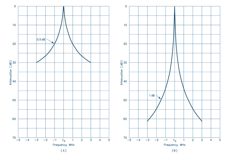
Only one coupling loop or probe is required for this method of filtering. This type of cavity could be used in the receiver line to "notch" the transmitter signal. Several cavities can be connected in series or parallel to increase the attenuation in a given configuration. The diagram below show the attenuation of a single cavity (A) and a pair of cavities (B).

The only situation in which cavity filters would not help is the case where the off-frequency noise of the transmitter was right on the receiver frequency. With cavity resonators, an important point to remember is that addition of a cavity across a transmission line may change the impedance of the system. This change can be compensated by adding tuning stubs along the transmission line.


Duplexers

Most amateur repeaters in the 144, 220 and 440 MHz bands use duplexers to obtain the necessary transmitter to receiver isolation. Duplexers have been commonly used in commercial repeaters for many years.

The duplexer consists of two high-Q filters. One filter is used in the feed line from the transmitter to the antenna, and another between the antenna and the receiver. These filters must have low loss at the frequency to which they are tuned while having very high attenuation at the surrounding frequencies. To meet the high attenuation requirements at frequencies within as little as 0.4% of the frequency to which they are tuned, the filters usually take the form of cascaded transmission line cavity filters.

These are either band-pass filters, or band-pass filters with a rejection notch which is tuned to the center frequency of the other filter. The number of cascaded filter sections is determined by the frequency separation and the ultimate attenuation requirements.

Duplexers for the amateur bands represent a significant technical challenge, because in most cases amateur repeaters operate with significantly less frequency separation than their commercial counterparts. Many manufacturers market high quality duplexers for the amateur frequencies.

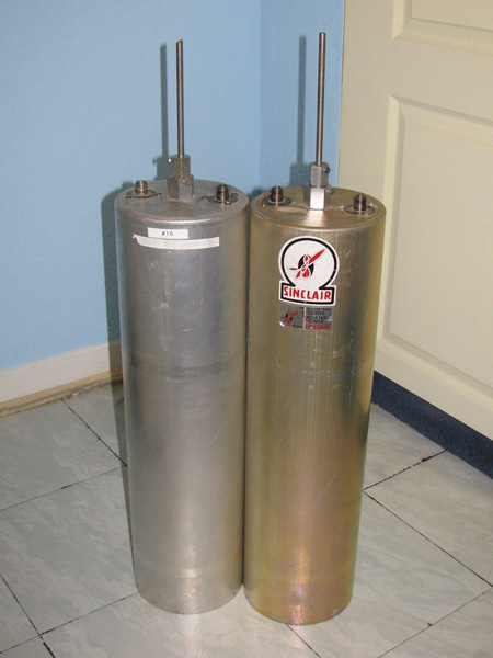
Duplexers consist of very high-Q cavities whose resonant frequencies are determined by mechanical components, in particular the tuning rod. The rod is usually made of a material that has a limited thermal expansion coefficient (such as Invar). Detuning of the cavity by environmental changes introduces unwanted losses in the antenna system.

These can be broken into four major categories:

• Ambient temperature variation (which leads to mechanical variations related to the thermal expansion coefficients of the materials used in the cavity).
• Humidity (dielectric constant) variation.
• Localized heating from the power dissipated in the cavity (resulting from its insertion loss).
• Mechanical variations resulting from other factors (vibration, etc).

In addition, because of the high-Q nature of these cavities, the insertion loss of the duplexer increases when the signal is not at the peak of the filter response. This means, in practical terms, that less power is radiated for a given transmitter output power.

Also, the drift in cavities in the receiver line results in increased system noise figure, reducing the sensitivity of the repeater. As the frequency separation between the receiver and the transmitter decreases, the insertion loss of the duplexer reaches certain practical limits. At 144 MHz, the minimum insertion loss for 600 kHz spacing is 1.5 dB per filter.

Testing and using duplexers requires some special considerations (especially as frequency increases). Because duplexers are very high-Q devices, they are very sensitive to the termination impedances at their ports. A high SWR on any port is a serious problem, because the apparent insertion loss of the duplexer will increase, and the isolation may appear to decrease. Some have found that when duplexers are used at the limits of their isolation capabilities, a small change in antenna SWR is enough to cause receiver desensitization. This occurs most often under ice-loading conditions on antennas with open-wire phasing sections.

The choice of connectors in the duplexer system is important. BNC connectors are good for use below 300 MHz. Above 300 MHz, their use is discouraged because even though many types of BNC connectors work well up to 1 GHz, older style standard BNC connectors are inadequate at UHF and above.

Type N connectors should be used above 300 MHz. It is false economy to use marginal quality connectors. Some commercial users have reported deteriorated isolation in commercial UHF repeaters when using such connectors. The location of a bad connector in a system is a complicated and frustrating process. Despite all these considerations, the duplexer is still the best method for obtaining isolation in the 144 - 925 MHz range.

Source: the ARRL Antenna Handbook

Coronal mass ejection heading our way

An active sunspot erupted Thursday, Jan. 19th, producing an M3-class solar flare and a full-halo coronal mass ejection (CME). The Solar and Heliospheric Observatory recorded the cloud expanding almost directly toward Earth.
Analysts at the Goddard Space Weather Lab say strong geomagnetic storms are possible when the cloud arrives this weekend. Their animated forecast track predicts an impact on Jan. 21st at 22:30 UT (+/- 7 hrs).

Electra Proximity Payload :: SDR ( software-defined radio) by NASA's Jet Propulsion Laboratory

Today, I stumbled upon a little SDR (software-defined radio) package with a big responsibility.

Electra Proximity Payload, is a software-defined radio defined and implemented by the Jet Propulsion Laboratory for use between spacecraft. It is typically used by a lander to communicate with an orbiter that can then communicate with Earth.

Click here to download the complete specifications in PDF format

Sources: Wikipedia and NASA

Multiband Dipole Antenna

Click on the image to enlarge it

This antenna system consists of a group of center-fed dipoles, all connected in parallel at the point where the transmission line joins them. The dipole elements are stagger-tuned. That is, they are individually cut to be λ/2 at different frequencies.

An extension of the stagger tuning idea is to construct multi-wire dipoles cut for different bands.
In theory, the 4-wire antenna of Fig 14 can be used with a coaxial feeder on five bands. The four wires are prepared as parallel-fed dipoles for 3.5, 7, 14, and 28 MHz. The 7-MHz dipole can be operated on its 3rd harmonic for 21-MHz operation to cover a fifth band. However, in practice it has been found difficult to get a good match to coaxial line on all bands.

The λ/2 resonant length of any one dipole in the presence of the others is not the same as for a dipole by itself due to interaction, and attempts to optimize all four lengths can become a frustrating procedure.
The problem is compounded because the optimum tuning changes in a different antenna environment, so what works for one amateur may not work for another. Even so, many amateurs with limited antenna space are willing to accept the mismatch on some bands just so they can operate on those frequencies using a single coax feed line.

Since this antenna system is balanced, it is desirable to use a balanced transmission line to feed it. The most desirable type of line is 75-ohm transmitting twin-lead. However, either 52-ohm or 75-ohm coaxial line can be used. Coax line introduces some unbalance, but this is tolerable on the lower frequencies. An alternative is to use a balun at the feed point, fed with coaxial cable.

The separation between the dipoles for the various frequencies does not seem to be especially critical. One set of wires can be suspended from the next larger set, using insulating spreaders (of the type used for feeder spreaders) to give a separation of a few inches. Users of this antenna often run some of the dipoles at right angles to each other to help reduce interaction. Some operators use inverted-V mounted dipoles as guy wires for the mast that supports the antenna system.

An interesting method of construction used successfully by Louis Richard, ON4UF, is shown below.
The antenna has four dipoles (for 7, 14, 21 and 28 MHz) constructed from 300-ohm ribbon transmission line. A single length of ribbon makes two dipoles. Thus, two lengths, as shown in the sketch, serve to make dipoles for four bands. Ribbon with copper-clad steel conductors (Amphenol type 14-022) should be used because all of the weight, including that of the feed line, must be supported by the uppermost wire. Two pieces of ribbon are first cut to a length suitable for the two halves of the longest dipole.
Then one of the conductors in each piece is cut to proper length for the next band higher in frequency. The excess wire and insulation is stripped away. A second pair of lengths is prepared in the same manner, except that the  lengths are appropriate for the next two higher frequency bands.

Click on the image to enlarge it

A piece of thick polystyrene sheet drilled with holes for anchoring each wire serves as the central insulator. The shorter pair of dipoles is suspended the width of the ribbon below the longer pair by clamps also made of poly sheet. Intermediate spacers are made by sawing slots in pieces of poly sheet so they will fit the ribbon snugly. The multiple-dipole principle can also be applied to vertical antennas. Parallel or fanned λ/4 elements of wire or tubing can be worked against ground or tuned radials from a common feed point.

Source: The ARRL Antenna Handbook

The J-Pole Antenna

Click on the image to enlarge it

The J-Pole is a half-wave antenna that is end-fed at its bottom. Since the radiator is longer than that of a 1/4-wave ground-plane antenna, the vertical lobe is compressed down toward the horizon and it has about 1.5 dB of gain compared to the ground-plane configuration.

The stub-matching section used to transform the high impedance seen looking into a half-wave to 50 Ω coax is shorted at the bottom, making the antenna look like the letter “J,” and giving the antenna its name.  Rigid copper tubing, fittings and assorted hardware can be used to make a really rugged J-pole antenna for 2 meters. When copper tubing is used, the entire assembly can be soldered together, ensuring electrical integrity, and making the whole antenna weatherproof.

No special hardware or machined parts are used in this antenna, nor are insulating materials needed, since the antenna is always at dc ground. Best of all, even if the parts aren’t on sale, the antenna can be built for less than $15. If you only build one antenna, you’ll have enough tubing left over to make most of a second antenna.

Construction
Copper and brass is used exclusively in this antenna. These metals get along together, so dissimilar metal corrosion is eliminated. Both metals solder well, too.

Cut the copper tubing to the lengths indicated. Item 9 is a 11/4-inch nipple cut from the 20-inch length of 1/2-inch tubing. This leaves 183/4 inches for the 1/4-matching stub. Item 10 is a 31/4-inch long nipple cut from the 60-inch length of 3/4-inch tubing. The 3/4-wave element should measure 563/4-inches long.

Remove burrs from the ends of the tubing after cutting, and clean the mating surfaces with sandpaper, steel wool, or emery cloth. After cleaning, apply a very thin coat of flux to the mating elements and assemble the tubing, elbow, tee, end caps and stubs. Solder the assembled parts with a propane torch and rosin-core solder. Wipe off excess solder with a damp cloth, being careful not to burn yourself.

The copper tubing will hold heat for a long time after you’ve finished soldering. After soldering, set the assembly aside to cool. Flatten one each of the 1/2-inch and 3/4-inch pipe clamps. Drill a hole in the flattened clamp as shown. Assemble the clamps and cut off the excess metal from the flattened clamp using the unmodified clamp as a template. Disassemble the clamps. Assemble the 1/2-inch clamp around the 1/4-wave element and secure with two of the screws, washers, and nuts as shown. Do the same with the 3/4-inch clamp around the 3/4-wave element. Set the clamps initially to a spot about 4 inches above the bottom of the “J” on their respective elements. Tighten the clamps only finger tight, since you’ll need to move them when tuning.

Tuning
The J-Pole can be fed directly from 50-ohm coax through a choke balun (3 turns of the feed coax rolled into a coil about 8 inches in diameter and held together with electrical tape). Before tuning, mount the antenna vertically, about 5 to 10 feet from the ground. A short TV mast on a tripod works well for this purpose.

When tuning VHF antennas, keep in mind that they are sensitive to nearby objects—such as your body. Attach the feed line to the clamps on the antenna, and make sure all the nuts and screws are at least finger tight. It really doesn’t matter to which element (¾-wave element or stub) you attach the coaxial center lead.

Tune the antenna by moving the two feed-point clamps equal distances a small amount each time until the SWR is minimum at the desired frequency. The SWR will be close to 1:1.

Final Assembly
The final assembly of the antenna will determine its long-term survivability. Perform the following steps with care. After adjusting the clamps for minimum SWR, mark the clamp positions with a pencil and then remove the feed line and clamps. Apply a very thin coating of flux to the inside of the clamp and the corresponding surface of the antenna element where the clamp attaches. Install the clamps and tighten the clamp screws.

Solder the feed line clamps where they are attached to the antenna elements. Now, apply a small amount of solder around the screw heads and nuts where they contact the clamps. Don’t get solder on the screw threads! Clean away excess flux with a non-corrosive solvent.

After final assembly and erecting/mounting the antenna in the desired location, attach the feed line and secure with the remaining washer and nut. Weather-seal this joint with RTV.

Source: The ARRL Antenna Handbook

About vacuum power tubes, by Matt Erickson KK5DR

Alex VE2VEH found this very good article on vacuum power tubes by Matt Erickson KK5DR.

Source: Matt Erickson's website

The G5RV Multiband HF Antenna

A multiband antenna that does not require a lot of space, is simple to construct, and is low in cost is the G5RV.

Designed in England by Louis Varney (G5RV) some years ago, it has become quite popular in the US. The G5RV design is shown in Fig 8. The antenna may be used from 3.5 through 30 MHz. Although some amateurs claim it may be fed directly with 50-Ω coax on several amateur bands with a low SWR, Varney himself recommended the use of an antenna tuner on bands other than 14 MHz. In fact, an analysis of the G5RV feed-point impedance shows there is no length of balanced line of any characteristic impedance that will transform the terminal impedance to the 50 to 75-Ω range on all bands. (Low SWR indication with coax feed and no matching network on bands other than 14 MHz may indicate excessive losses in the coaxial line.)

Fig 2 shows the 20-meter azimuthal pattern for a G5RV at a height of 50 feet over fl at ground, at an elevation angle of 5° that is suitable for DX work. For comparison, the response for two other antennas is also shown in Fig 2—a standard half wave 20-meter dipole at 50 feet and a 132-foot long center-fed dipole at 50 feet.

The G5RV on 20 meters is, of course, longer than a standard half wave dipole and it exhibits about 2 dB more gain compared to that dipole. With four lobes making it look rather like a four-leaf clover, the azimuth pattern is more omni directional than the two-lobed dipole. The 132-foot center-fed dipole is longer than the G5RV and it has about 0.5 dB more gain than the G5RV, also exhibiting four major lobes, along with two strong minor lobes in the plane of the wire. Overall, the azimuthal response for the G5RV is more omni directional than the comparison antennas.

The G5RV patterns for other frequencies are similar to those shown for the 135-foot dipole previously for other frequencies. Incidentally, you may be wondering why a 132-foot dipole is shown in Fig 2, rather than the 135-foot dipole described earlier.

The portion of the G5RV antenna shown as horizontal in Fig 1 may also be installed in an inverted-V dipole arrangement, subject to the same loss of peak gain mentioned above for the 135-foot dipole. Or instead, up to 1⁄6 of the total length of the antenna at each end may be dropped vertically, semi-vertically, or bent at a convenient angle to the main axis of the antenna, to cut down on the requirements for real estate.

Fig. 1

The G5RV multiband antenna covers 3.5 through 30 MHz. Although many amateurs claim it may be fed directly with 50-Ω coax on several amateur bands, Louis Varney, its originator, recommends the use of a matching network on bands other than 14 MHz.

Fig. 2

Azimuth pattern at a 5° takeoff angle for a 102-foot long, 50-foot high G5RV dipole (solid line). For comparison, the response for a 132-foot long, center-fed dipole at 50 feet height (dashed line) and a 33-foot long half wave 20-meter dipole at 50 feet (dotted line) are also shown. The longest antenna exhibits about 0.5 dB more gain than the G5RV, although the response is more omnidirectional for the G5RV—an advantage for a wire antenna that is not usually rotatable.


Source: ARRL Antenna Handbook 2010

Simple HF Antennas

The simplest multiband antenna is a random length of #12 or #14 wire. Power can be fed to the wire on practically any frequency using one or the other of the methods shown in Fig 1. If the wire is made either 67 or 135 feet long, it can also be fed through a tuned circuit, as in Fig 2. It is advantageous to use an SWR bridge or other indicator in the coax line at the point marked “X.”

If you have installed a 28- or 50-MHz rotary beam, in many cases it may be possible to use the beam’s feed line as an antenna on the lower frequencies. Connecting the two wires of the feeder together at the station end will give a random length wire that can be conveniently coupled to the transmitter as in Fig 1. The rotary system at the far end will serve only to end-load the wire and will not have much other effect.

One disadvantage of all such directly fed systems is that part of the antenna is practically within the station, and there is a good chance that you will have some trouble with RF feedback. RF within the station can often be minimized by choosing a length of wire so that the low feed-point impedance at a current loop occurs at or near the transmitter. This means using a wire length of λ/4 (65 feet at 3.6 MHz, 33 feet at 7.1 MHz), or an odd multiple of λ/4 (3⁄4-λ is 195 feet at 3.6 MHz, 100 feet at 7.1 MHz).

Obviously, this can be done for only one band in the case of even harmonically related bands, since the wire length that presents a current loop at the transmitter will present a voltage loop at two (or four) times that frequency.

When you operate with a random-length wire antenna, as in Figs 1 and 2, you should try different types of grounds on the various bands, to see what gives you the best results. In many cases it will be satisfactory to return to the transmitter chassis for the ground, or directly to a convenient metallic water pipe. If neither of these works well (or the metallic water pipe is not available), a length of #12 or #14 wire (approximately λ/4 long) can often be used to good advantage. Connect the wire at the point in the circuit that is shown grounded, and run it out and down the side of the house, or support it a few feet above the ground if the station is on the first floor or in the basement. It should not be connected to actual ground at any point.

Fig 1 - At A, a random-length wire driven directly from the pi-network output of a transmitter. At B, an L network for use in cases where sufficient loading cannot be obtained with the arrangement at A. C1 should have about the same plate spacing as the final tank capacitor in a vacuum-tube type of transmitter; a maximum capacitance of 100 pF is sufficient if L1 is 20 to 25 μH. A suitable coil would consist of 30 turns of #12 wire, 2½ inches diameter, 6 turns per inch. Bare wire should be used so the tap can be placed as required for loading the transmitter.

Fig 2 - If the antenna length is 137 feet, a parallel-tuned coupling circuit can be used on each amateur band from 3.5 through 30 MHz, with the possible exception of the WARC 10-, 18- and 24-MHz bands. C1 should duplicate the final tank tuning capacitor and L1 should have the same dimensions as the final tank inductor on the band being used. If the wire is 67 feet long, series tuning can be used on 3.5 MHz as shown at the left; parallel tuning will be required on 7 MHz and higher frequency bands. C2 and L2 will in general duplicate the final tank tuning capacitor and inductor, the same as with parallel tuning. The L network shown in Fig 1B is also suitable for these antenna lengths.



Source: ARRL Antenna Handbook 2010

HRS Antennas

HRS antennas were invented during the 1920s and 1930s when there was a lot of experimentation with long distance shortwave broadcasting

The Distributed or Branch Feed curtains are considered to be classical HRS type antennas. There are 4 mathematical model types of ITU HRS type HF antennas.

Distributed or Branch Feed curtain arrays are called HR type curtain arrays. The H and R standing for Height and Rows. When they are steerable, they are sometimes called HRS arrays, the S representing "steerable".

An HR 4/3 would be an antenna 4 elements high and 3 elements wide. If it was an HRS 4/3, it would be a steerable array of the same element configuration.

The HRS antenna type was not originally intended for voice and music broadcasting. However, the directional properties of this antenna type were ideal for voice broadcasting—and the design is now pervasive in international broadcasting by the 1950s. As far back as the mid-1930s, Radio Netherlands was using a rotatable HRS antenna for global coverage.

Read the full article on Wikipedia